Vector Kinematics

Kinematics describes motion without considering the forces that cause it. In mechanics and robotics, it provides the tools needed to describe position, velocity, and acceleration of points in moving reference frames.

Note

This page assumes familiarity with reference frames and rotation matrices. See Reference frames for a full introduction including unit vectors, rotation matrix derivations, and Euler angle conventions.

Reference frames and position

\(\mathbf{r}_{P/O} = \mathbf{r}_{O_b/O} + \mathbf{r}_{P/O_b}\)

\(\mathbf{r}_{O_b/O}\) \(\mathbf{r}_{P/O_b}\) \(\mathbf{r}_{P/O}\)

Pause

Consider a fixed inertial frame \(i\) and a moving body frame \(b\) that may translate and rotate relative to \(i\). A point \(P\) fixed in \(b\) may still move relative to \(i\) because the frame itself moves.

The position of \(P\) relative to the origin \(O\) of the fixed frame decomposes as

(54)\[\vec{r}_{P/O} = \vec{r}_{O_b/O} + \vec{r}_{P/b}\]

All vectors in this sum must be expressed in the same frame before they can be added numerically.

Rotation transformations

If \(\mathbf{r}^b\) is a vector expressed in frame \(b\), its coordinates in frame \(0\) are obtained by

(55)\[\mathbf{r}^0 = R^0_b \, \mathbf{r}^b\]

The three principal rotation matrices are

(56)\[\begin{split}R_z(\psi) = \begin{pmatrix} \cos\psi & -\sin\psi & 0 \\ \sin\psi & \cos\psi & 0 \\ 0 & 0 & 1 \end{pmatrix} \qquad R_y(\theta) = \begin{pmatrix} \cos\theta & 0 & \sin\theta \\ 0 & 1 & 0 \\ -\sin\theta & 0 & \cos\theta \end{pmatrix} \qquad R_x(\phi) = \begin{pmatrix} 1 & 0 & 0 \\ 0 & \cos\phi & -\sin\phi \\ 0 & \sin\phi & \cos\phi \end{pmatrix}\end{split}\]

An arbitrary orientation can be built by composing these. A common choice for ships, aircraft, and drones is the ZYX (yaw, pitch, roll) sequence

(57)\[R^0_b = R_z(\psi)\,R_y(\theta)\,R_x(\phi)\]

See Reference frames for the derivation of these matrices and a discussion of intrinsic versus extrinsic rotation conventions.

Exercise: Coordinate transformation using a rotation matrix

A drone’s body frame \(b\) is obtained from the inertial frame by a pure yaw rotation of \(\psi = 90°\) followed by a pure pitch rotation of \(\theta = 30°\). The combined rotation matrix is

(58)\[R^0_b = R_z(90°)\,R_y(30°)\]

A velocity vector is measured by an onboard sensor and expressed in the body frame as

(59)\[\begin{split}\mathbf{v}^b = \begin{pmatrix} 2 \\ 0 \\ -1 \end{pmatrix} \text{ m/s}\end{split}\]

Find the same velocity expressed in the inertial frame \(\mathbf{v}^0\).

Solution

First, evaluate the two principal rotation matrices.

Yaw (\(\psi = 90°\), so \(\cos 90° = 0\), \(\sin 90° = 1\)):

(60)\[\begin{split}R_z(90°) = \begin{pmatrix} 0 & -1 & 0 \\ 1 & 0 & 0 \\ 0 & 0 & 1 \end{pmatrix}\end{split}\]

Pitch (\(\theta = 30°\), so \(\cos 30° = \tfrac{\sqrt{3}}{2}\), \(\sin 30° = \tfrac{1}{2}\)):

(61)\[\begin{split}R_y(30°) = \begin{pmatrix} \tfrac{\sqrt{3}}{2} & 0 & \tfrac{1}{2} \\ 0 & 1 & 0 \\ -\tfrac{1}{2} & 0 & \tfrac{\sqrt{3}}{2} \end{pmatrix}\end{split}\]

Combined rotation:

(62)\[\begin{split}R^0_b = R_z(90°)\,R_y(30°) = \begin{pmatrix} 0 & -1 & 0 \\ 1 & 0 & 0 \\ 0 & 0 & 1 \end{pmatrix} \begin{pmatrix} \tfrac{\sqrt{3}}{2} & 0 & \tfrac{1}{2} \\ 0 & 1 & 0 \\ -\tfrac{1}{2} & 0 & \tfrac{\sqrt{3}}{2} \end{pmatrix} = \begin{pmatrix} 0 & -1 & 0 \\ \tfrac{\sqrt{3}}{2} & 0 & \tfrac{1}{2} \\ -\tfrac{1}{2} & 0 & \tfrac{\sqrt{3}}{2} \end{pmatrix}\end{split}\]

Transform the vector:

(63)\[\begin{split}\mathbf{v}^0 = R^0_b\,\mathbf{v}^b = \begin{pmatrix} 0 & -1 & 0 \\ \tfrac{\sqrt{3}}{2} & 0 & \tfrac{1}{2} \\ -\tfrac{1}{2} & 0 & \tfrac{\sqrt{3}}{2} \end{pmatrix} \begin{pmatrix} 2 \\ 0 \\ -1 \end{pmatrix} = \begin{pmatrix} 0 \\ \sqrt{3} - \tfrac{1}{2} \\ -1 - \tfrac{\sqrt{3}}{2} \end{pmatrix} \approx \begin{pmatrix} 0 \\ 1.23 \\ -1.87 \end{pmatrix} \text{ m/s}\end{split}\]

The rotation changes the direction of the velocity vector but not its magnitude. In both frames \(\lVert\mathbf{v}\rVert = \sqrt{5}\) m/s.

Velocity in a moving frame

The velocity of point \(P\) relative to the inertial frame \(i\), expressed in \(i\), is

(64)\[\vec{v}_{P/i}^i = \vec{v}_{b/i}^i + \frac{d^b}{dt}\vec{r}_{P/b} + \vec{\omega}_{b/i}^i \times \vec{r}_{P/b}\]

The three terms each capture a distinct contribution to the motion of \(P\):

• \(\vec{v}_{b/i}^i\) is the translational velocity of the moving frame origin.

• \(\frac{d^b}{dt}\vec{r}_{P/b}\) is the velocity of \(P\) relative to the moving frame. It is zero when \(P\) is fixed in the body, for example a static sensor.

• \(\vec{\omega}_{b/i}^i \times \vec{r}_{P/b}\) is the velocity caused by the rotation of the frame. It is nonzero even when \(P\) is fixed in the body.

A note on the frame-dependent derivative

The notation \(\frac{d^b}{dt}\) means the derivative is taken while observing the vector from frame \(b\), where the basis vectors are fixed. Only changes in the coordinates of the vector contribute.

If \(P\) is fixed in the body frame, its coordinates in \(b\) are constant, so

(65)\[\frac{d^b}{dt}\vec{r}_{P/b} = \mathbf{0}\]

When the same vector is viewed from the inertial frame, it still appears to change because the frame rotates. That effect is captured separately by the third term \(\vec{\omega}_{b/i}^i \times \vec{r}_{P/b}\).

The animations below illustrate the three terms acting simultaneously, first for a generic rigid body and then for a ship.

1. Frame translation

Only the translation of frame b relative to frame i is shown.

2. Relative motion in frame b

The point moves relative to frame b.

3. Frame rotation

The point is fixed in frame b, but frame b rotates.

4. Combined motion

Only the total velocity of P in the inertial frame is shown.

1. Boat translation

Only the translation of the boat relative to the inertial frame is shown.

2. Relative motion on deck

The person moves relative to the boat.

3. Boat rotation

The person is fixed on deck, but the boat rotates.

4. Combined motion

Only the total velocity of P in the inertial frame is shown.

Exercise: Velocity of a point on a rotating vessel

A ship (body frame \(b\)) moves through calm water with a constant translational velocity \(\vec{v}_{b/i}^i = (3, 1, 0)^\top\) m/s expressed in the inertial frame. The ship rotates at a constant yaw rate \(\dot\psi = 0.2\) rad/s about the vertical axis, so the angular velocity is \(\vec{\omega}_{b/i}^i = (0, 0, 0.2)^\top\) rad/s.

A sensor is mounted on the bow, fixed to the ship at position \(\vec{r}_{P/b}^b = (5, 0, 0)^\top\) m (5 m ahead of the ship origin along the body x-axis).

At the instant of interest the body frame coincides with the inertial frame (\(R^0_b = I\)), so \(\vec{r}_{P/b}^i = (5, 0, 0)^\top\) m.

Find the velocity of the sensor relative to the inertial frame at this instant.

Solution

Because the sensor is fixed in the body frame, the relative velocity term vanishes:

(66)\[\frac{d^b}{dt}\vec{r}_{P/b} = \mathbf{0}\]

The velocity equation reduces to

(67)\[\vec{v}_{P/i}^i = \vec{v}_{b/i}^i + \vec{\omega}_{b/i}^i \times \vec{r}_{P/b}^i\]

Compute the cross product:

(68)\[\begin{split}\vec{\omega}_{b/i}^i \times \vec{r}_{P/b}^i = \begin{pmatrix} 0 \\ 0 \\ 0.2 \end{pmatrix} \times \begin{pmatrix} 5 \\ 0 \\ 0 \end{pmatrix} = \begin{pmatrix} 0 \cdot 0 - 0.2 \cdot 0 \\ 0.2 \cdot 5 - 0 \cdot 0 \\ 0 \cdot 0 - 0 \cdot 5 \end{pmatrix} = \begin{pmatrix} 0 \\ 1 \\ 0 \end{pmatrix} \text{ m/s}\end{split}\]

Adding the translational velocity:

(69)\[\begin{split}\vec{v}_{P/i}^i = \begin{pmatrix} 3 \\ 1 \\ 0 \end{pmatrix} + \begin{pmatrix} 0 \\ 1 \\ 0 \end{pmatrix} = \begin{pmatrix} 3 \\ 2 \\ 0 \end{pmatrix} \text{ m/s}\end{split}\]

The rotation adds 1 m/s in the \(y\)-direction because the bow sweeps sideways as the ship yaws.

Acceleration in a moving frame

To find the acceleration, differentiate the velocity equation with respect to time in the inertial frame. The key tool is the transport theorem: for any vector \(\vec{u}\),

(70)\[\frac{d^i}{dt}\vec{u} = \frac{d^b}{dt}\vec{u} + \vec{\omega}_{b/i} \times \vec{u}\]

Applying this to each term in the velocity equation and collecting gives

(71)\[\vec{a}_{P/i}^i = \vec{a}_{b/i}^i + \left(\vec{a}_P\right)_b + \vec{\alpha}_{b/i}^i \times \vec{r}_{P/b} + \vec{\omega}_{b/i}^i \times \left(\vec{\omega}_{b/i}^i \times \vec{r}_{P/b}\right) + 2\,\vec{\omega}_{b/i}^i \times \frac{d^b}{dt}\vec{r}_{P/b}\]

Each term has a clear physical meaning:

• \(\vec{a}_{b/i}^i\) is the acceleration of the moving frame origin.

• \(\left(\vec{a}_P\right)_b\) is the acceleration of \(P\) relative to the moving frame.

• \(\vec{\alpha}_{b/i}^i \times \vec{r}_{P/b}\) is the tangential acceleration caused by angular acceleration of the frame.

• \(\vec{\omega}_{b/i}^i \times \left(\vec{\omega}_{b/i}^i \times \vec{r}_{P/b}\right)\) is the centripetal acceleration, always directed toward the rotation axis.

• \(2\,\vec{\omega}_{b/i}^i \times \frac{d^b}{dt}\vec{r}_{P/b}\) is the Coriolis acceleration, which arises when \(P\) moves within a rotating frame.

The animation below shows the two most commonly encountered terms: centripetal (panel 1) and Coriolis (panel 2).

1. Centripetal acceleration

+ −

\(P\) is fixed in the rotating frame. The centripetal term \(\boldsymbol{\omega}\times(\boldsymbol{\omega}\times\mathbf{r}_{P/b})\) always points inward toward the rotation axis.

2. Coriolis acceleration

+ −

\(P\) slides along the rotating arm. The Coriolis term \(2\boldsymbol{\omega}\times\tfrac{d^b}{dt}\mathbf{r}_{P/b}\) acts perpendicular to the sliding motion.

Summary

The key ideas of vector kinematics are:

• Vectors must be expressed in a common frame before they can be added.

• Rotation matrices transform coordinates between frames. See Reference frames for derivations and Euler angle conventions.

• A rotating frame induces an extra velocity term \(\vec{\omega} \times \vec{r}\) even for points fixed in the body.

• Differentiating the velocity equation via the transport theorem yields five acceleration terms, including centripetal and Coriolis contributions.

These ideas are fundamental in rigid-body mechanics, robotics, and vehicle dynamics.

A modern cautionary tale

In 2026, a French sailor reportedly revealed the position of the aircraft carrier \(\textit{Charles de Gaulle}\) by uploading a public Strava run recorded on the deck.

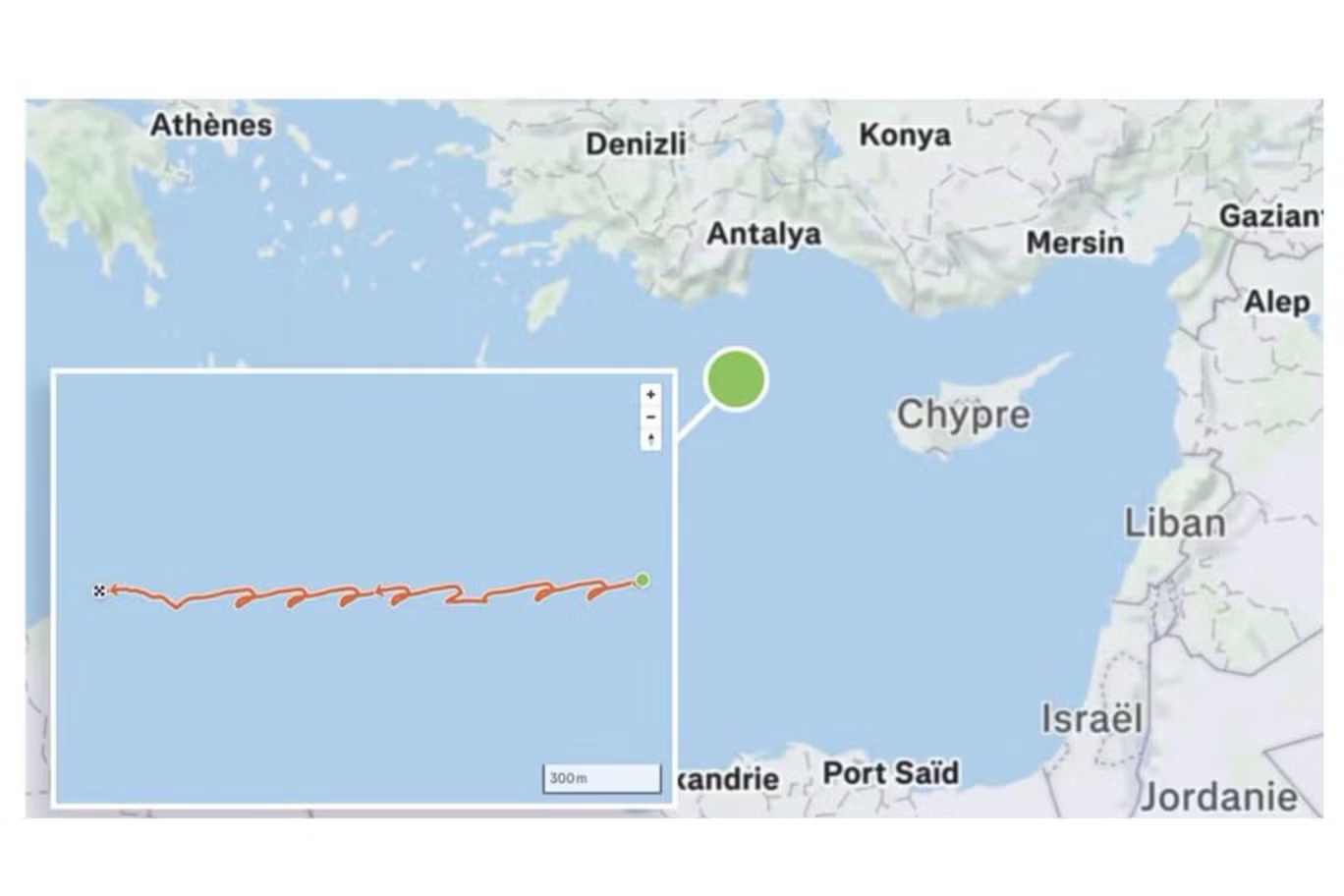
Fig. 11 A recorded trajectory can reveal the motion of the entire reference frame.

Vector kinematics with SymPy mechanics

sympy.physics.mechanics lets you work with symbolic reference frames, points, and vectors. Orientations between frames are declared once; SymPy then differentiates vectors in the correct frame when you ask for velocities and accelerations.

Setting up frames and orientation

import sympy as sm
from sympy.physics.mechanics import ReferenceFrame, Point, dynamicsymbols
sm.init_printing(use_latex='mathjax')

psi, v_x, v_y = dynamicsymbols("psi v_x v_y")

N = ReferenceFrame("N")  # inertial frame
B = N.orientnew("B", "Axis", [psi, N.z])  # body frame: yaw by psi about N.z

B.ang_vel_in(N)

\[\displaystyle \frac{d}{d t} \psi{\left(t \right)}\mathbf{\hat{n}_z}\]

The prime denotes \(d/dt\), so the result is \(\vec\omega_{B/N} = \dot\psi\,\hat{N}_z\).

Velocity via the two-point theorem

v2pt_theory(Q, N, B) sets the velocity of a point using the transport theorem, given the velocity of a reference point Q and assuming both points are fixed in frame B:

O = Point("O")  # inertial origin (fixed)
O_b = Point("O_b")  # ship origin

O.set_vel(N, 0)
O_b.set_vel(N, v_x * N.x + v_y * N.y)

P = O_b.locatenew("P", 5 * B.x)  # bow sensor, 5 m along body x-axis
P.v2pt_theory(O_b, N, B)

P.vel(N)

\[\displaystyle v_{x}{\left(t \right)}\mathbf{\hat{n}_x} + v_{y}{\left(t \right)}\mathbf{\hat{n}_y} + 5 \frac{d}{d t} \psi{\left(t \right)}\mathbf{\hat{b}_y}\]

Substituting \(\psi = 0\), \(\dot\psi = 0.2\) rad/s, \(v_x = 3\) m/s, \(v_y = 1\) m/s recovers the result from the exercise above:

P.vel(N).subs({psi: 0, psi.diff(): 0.2, v_x: 3, v_y: 1}).to_matrix(N)

\[\begin{split}\displaystyle \left[\begin{matrix}3 - 1.0 \sin{\left(\psi{\left(t \right)} \right)}\\1.0 \cos{\left(\psi{\left(t \right)} \right)} + 1\\0\end{matrix}\right]\end{split}\]

Acceleration

acc() differentiates the stored velocity, applying the transport theorem again to produce all five terms from the acceleration formula, including centripetal and Coriolis:

P.acc(N).express(N).simplify()

\[\displaystyle (- 5 \sin{\left(\psi{\left(t \right)} \right)} \frac{d^{2}}{d t^{2}} \psi{\left(t \right)} - 5 \cos{\left(\psi{\left(t \right)} \right)} \left(\frac{d}{d t} \psi{\left(t \right)}\right)^{2} + \frac{d}{d t} v_{x}{\left(t \right)})\mathbf{\hat{n}_x} + (- 5 \sin{\left(\psi{\left(t \right)} \right)} \left(\frac{d}{d t} \psi{\left(t \right)}\right)^{2} + 5 \cos{\left(\psi{\left(t \right)} \right)} \frac{d^{2}}{d t^{2}} \psi{\left(t \right)} + \frac{d}{d t} v_{y}{\left(t \right)})\mathbf{\hat{n}_y}\]

Vectors can be expressed in any frame with .express() and converted to a column matrix with .to_matrix().

Note

For more examples of rolling discs, pendulums, multi-body systems, and full equations of motion via Kane’s and Lagrange’s methods, see the SymPy mechanics documentation.