3D Visualization and Animation

Visualization is a crucial part of evaluating any attempt of modelling a system. When dealing with a system with more than a couple of parameters, plots become difficult to interpret. By visualizing our system in 3D we can leverage our spatial and physics intuition of the world. This is the same intuition which tells us that when we throw a ball, its trajectory should be parabolic, or the intuition that it takes less effort stop a bike than a car. When it comes to mechanical systems, when something doesn’t look right, it’s indicative of a model built on fundamentally flawed assumptions. Visualizing your system through animation will help you weed out unintended behaviour from your model and will ultimately deepen your understanding of your model. This page will go into the basic principles of animating a system in 3D, as well as some common frameworks for visualization an animation.

Principles of Animation

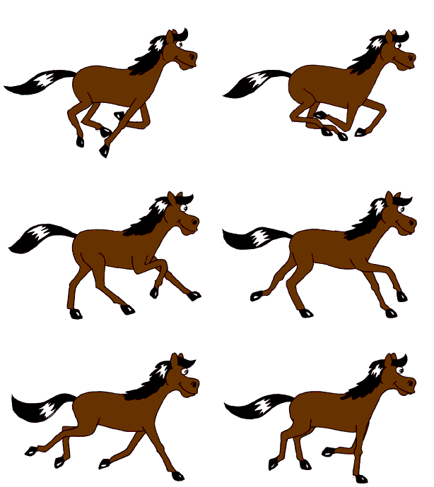
By Janke - Own work, CC BY-SA 2.5, Link

We distinguish between two approaches to animation: real-time animation and precomputed animation.

Real-time animation means that we simulate the system’s state in the same loop (as in programming) as the animation progress. For each new animation frame we integrate our system from the last frame to the current frame. This allows for interactive and responsive animations, but can be computationally demanding for complex systems or stiff systems that demand fine time resolutions.

Precomputed animation uses pre-generated trajectories (state over time). We compute the system’s trajectory before animating, and play back the trajectory upon animation. This approach is often more practical and efficient, as it allows us to decouple simulation from rendering. This allows us to reuse our simulation data, and is generally more stable for visualization purposes.

In both cases, we need a time series of the trajectory of our system. This trajectory could include positions, orientations and other relevant quantities and measures. Additionally, we need to specify the time step or frame duration between each state, as this determines how long each animation frame should last, consequently determining our frame rate (frames/second). Matching the animation frame rate with the simulation time step produces a reproduction of the system’s motion. However, in some cases adjusting the playback speed (faster or slower) can be both practically useful (i.e. a very slow or fast system).

A trajectory alone is not very useful to animate without a corresponding 3D (or 2D) model of the system. This model doesn’t need to be photorealistic nor physically accurate. It just needs to capture the essential geometry and behaviour of our system. For example, the details on the bike seat are of little interest when analysing the motion of a bike. Most animation libraries include primitive geometric shapes like cubes, spheres and cylinders, which are usually sufficient to represent the key components of a system. You’d be surprised how basic a model can be, as our brains are excellent at filling in the blanks when the motion is convincing. A simple rectangle moving like a boat can evoke the image of a vessel at sea given that the motion behaves as expected.

Our advice: start simple. Focus on correct motion first, as you undoubtedly will make some interesting mistakes with reference frames and defining coordinate systems. You can always improve the visual flair and fidelity later. The goal is by no means to produce a Pixar-quality animation, but rather to understand and effectively communicate how your system behaves.

In the following sections, we’ll present four animation tools of increasing complexity, from lightweight plotting using Matplotlib to state-of-the-art 3D engines using Blender.

Matplotlib.animation

Note

Matplotlib is quite old and rigorous for simple data visualization. If you want to plot simple 2D data, we recommend checking out Plotly for a more modern plotting library. However, Plotly it is not designed for 3D animation.

Many of you are already familiar with the Matplotlib library. Inspired by Matlab’s plotting library, Matplotlib offers many useful easy-to-use functions for plotting and visualizing data. While library was made with data visualization in mind, it also supports a rudimentary framework for plotting and animating in 3D. In this section we’ll go through a basic example of a 3D pendulum with damping. For a more comprehensive introduction to Matplotlib.animation, take a look at the official documentation.

Example: Pendulum

In this example we’ll simulate a 3D pendulum with damping terms.

Derivation

We consider a point mass \(m\) suspended by a rigid rod of length \(L\) from a fixed pivot. Using spherical coordinates, the generalized coordinates are

(2)\[\begin{split}q = \begin{bmatrix} \theta \\ \phi \end{bmatrix},\end{split}\]

where \(\theta\) is the polar angle from the vertical and \(\phi\) is the azimuthal angle around the vertical axis.

The position of the mass is \(\mathbf{r} = L(\sin\theta\cos\phi, \sin\theta\sin\phi, -\cos\theta)\). Computing the kinetic energy \(T = \tfrac{1}{2}m|\dot{\mathbf{r}}|^2\) gives us

(3)\[T = \tfrac{1}{2}mL^2\left[\dot{\theta}^2 + \sin^2\theta \, \dot{\phi}^2\right]\]

The potential energy, with reference at the pivot at the origin, is

(4)\[V = -mgL\cos\theta.\]

Thus, the Lagrangian can be expressed as

(5)\[\mathcal{L} = T - V.\]

The kinetic energy can be written in quadratic form

(6)\[T = \tfrac{1}{2} \dot{q}^\mathsf{T} W(q)\, \dot{q},\]

with inertia matrix

(7)\[\begin{split}W(q) = mL^2 \begin{bmatrix} 1 & 0 \\ 0 & \sin^2\theta \end{bmatrix}\end{split}\]

The Euler-Lagrange equations yield

(8)\[W(q) \, \ddot{q} + c(q, \dot{q}) + g(q) = 0,\]

where

(9)\[\begin{split}c(q, \dot{q}) = mL^2 \begin{bmatrix} -\sin\theta\cos\theta \, \dot{\phi}^2 \\ -2\cos\theta \, \dot{\theta}\dot{\phi} \end{bmatrix}, \qquad g(q) = \begin{bmatrix} mgL\sin\theta \\ 0 \end{bmatrix}.\end{split}\]

The final equations of motion are

(10)\[\begin{split}\begin{bmatrix} mL^2 & 0 \\ 0 & mL^2\sin^2\theta \end{bmatrix} \begin{bmatrix} \ddot{\theta} \\ \ddot{\phi} \end{bmatrix} + \begin{bmatrix} -mL^2\sin\theta\cos\theta \, \dot{\phi}^2 + mgL\sin\theta \\ -2mL^2\cos\theta \, \dot{\theta}\dot{\phi} \end{bmatrix} = 0.\end{split}\]

This compact form can be inverted to solve for \(\ddot{\theta}\) and \(\ddot{\phi}\) explicitly:

(11)\[\begin{split}\ddot{\theta} &= \sin\theta\cos\theta \, \dot{\phi}^2 - \frac{g}{L}\sin\theta \\ \ddot{\phi} &= -\frac{2\cos\theta}{\sin\theta} \dot{\theta}\dot{\phi}\end{split}\]

Adding damping terms \(-c\dot{\theta}\) and \(-c\dot{\phi}\), we finally have:

(12)\[\begin{split}\ddot{\theta} &= \sin\theta\cos\theta \, \dot{\phi}^2 - \frac{g}{L}\sin\theta - c\dot{\theta} \\ \ddot{\phi} &= -\frac{2\cos\theta}{\sin\theta} \dot{\theta}\dot{\phi} - c\dot{\phi}\end{split}\]

From Euler-Lagrange using vertical angle \(\theta\) and azimuth \(\phi\) as generalized coordinates we get the following EoM:

Note

This simplified damping model works for demonstration but isn’t fully realistic

(13)\[\begin{split}\ddot{\theta} &= \sin\theta\cos\theta \, \dot{\phi}^2 - \frac{g}{L}\sin\theta - c\dot{\theta} \\ \ddot{\phi} &= -\frac{2\cos\theta}{\sin\theta} \dot{\theta}\dot{\phi} - c\dot{\phi}\end{split}\]

We separate the second order ODE into four first order ODEs on the standard SciPy format. We also define our parameters.

import numpy as np

g, L = 9.81, 2.0
c = 0.5  # damping coeff

def spherical_pendulum_damped(t, y):
    theta, theta_dot, phi, phi_dot = y
    theta_ddot = (np.sin(theta)*np.cos(theta)*phi_dot**2
                  - (g/L)*np.sin(theta)
                  - c*theta_dot)
    phi_ddot = (-2*np.cos(theta)/max(np.sin(theta), 1e-6))*theta_dot*phi_dot - c*phi_dot # Numerical stability
    return [theta_dot, theta_ddot, phi_dot, phi_ddot]

Integrating with SciPy

from scipy.integrate import solve_ivp
# Initial conditions
theta0, theta_dot0 = 0.8, 0.0
phi0, phi_dot0 = 0.8, 2.0

# Integrate
t_span = (0, 10) # 10 seconds
t_eval = np.linspace(*t_span, 600) # Resolution
y0 = [theta0, theta_dot0, phi0, phi_dot0]
sol = solve_ivp(spherical_pendulum_damped, t_span, y0, t_eval=t_eval)

theta, phi = sol.y[0], sol.y[2] # Extract trajectory polar coordinates

Polar coordinates can be tricky to work with, so to make animation simpler we convert to Cartesian

x = L * np.sin(theta) * np.cos(phi)
y = L * np.sin(theta) * np.sin(phi)
z = -L * np.cos(theta)

Similar to an ordinary plot, we create a figure with plt.fig() and add a 3D subplot. We can also set the bounds of our plot explicitly by set_lim() for all axes.

import matplotlib.pyplot as plt

fig = plt.figure()
ax = fig.add_subplot(111, projection="3d")
ax.set_xlim(-L, L)
ax.set_ylim(-L, L)
ax.set_zlim(-L, 0.5*L)
ax.set_box_aspect([1, 1, 0.6]) # Not strictly necessary, but nice for web view

We’ve now created out plot. Now for the animation. The simplest way to animate using Matplotlib is to define a trajectory for every object in your system. We create one for the line (rod) and one for the bob (mass attached to rod). Like any other plot we can pick the formatting for each of the trajectories.

line, = ax.plot([], [], [], lw=2, c="black") # The comma "," unpacks the one-element list returned by ax.plot()
bob, = ax.plot([], [], [], "o", c="red", markersize=8)

We’ll now define the functions we need to animate the trajectory using FuncAnimation. Apart from our figure and data, the animation function needs an initialization function and an update function to animate our trajectory. The initialization function sets up all the properties we need for the trajectories we animate, and gets called whenever we reset or restart our animation. The update function takes in which time step we are on, and returns the updated trajectory of the objects we animate.

That’s it!

def init():
    line.set_data([], [])
    line.set_3d_properties([])
    bob.set_data([], [])
    bob.set_3d_properties([])
    return line, bob

def update(i):
    line.set_data([0, x[i]], [0, y[i]])
    line.set_3d_properties([0, z[i]])
    bob.set_data([x[i]], [y[i]])
    bob.set_3d_properties([z[i]])
    return line, bob

Then we just have to pass our figure, functions and remaining parameters. The frame argument is the number of steps we integrated is self explanatory. The interval parameter controls milliseconds between frames, use 50-100ms for smooth playback. Additionally, you can use blit=True to make the animation more efficient, as it makes sure only updated pixels are drawn for every frame. If the animation doesn’t appear when testing locally, try removing blit=True or use plt.show() instead of HTML display.

from matplotlib.animation import FuncAnimation
from IPython.display import HTML # HTML needed to display on webpage

ani = FuncAnimation(fig, update, frames=len(t_eval), init_func=init,
                    blit=True, interval=10)

plt.close(fig)  # suppress static plot, animate using HTML instead
HTML(ani.to_jshtml()) # Display inline

Once Loop Reflect

Alternative display methods include plt.show() for interactive viewing or ani.save(‘pendulum.mp4’) to save as video. Matplotlib animations may behave differently depending on your backend. If the animation doesn’t display properly, try switching backends before importing pyplot:

import matplotlib
matplotlib.use('TkAgg')  # or 'Qt5Agg', 'notebook' for Jupyter
import matplotlib.pyplot as plt

Common backends include TkAgg for desktop applications, Qt5Agg for interactive plots and ‘notebook’ for Jupyter environments, such as Jupyter notebooks.

Pythreejs

Warning

This is a sparsely maintained Python package. It’s simple to use, but since compatibility is not guaranteed, use it at your own risk.

Pythreejs is a Jupyter widgets based notebook extension (library made specifically for Jupyter notebooks) that makes it possible to use some of the capabilities of the widely popular 3D animation framework threejs. From the name you probably figured out that threejs is written in Javascript. Since we use Python in this course we’ll introduce threejs through pythreejs first, and then take a look at threejs. In this section we’ll go through a simple example using pythreejs. We’ll introduce concepts such as scenes, cameras and much more.

Example: Pendulum-cart

The example system we’ll be animating is a cart pendulum with a mass or bob attached at the end, as shown in Cart with pendulum [Gro11]). We’ll ignore collision and friction forces for now.

Fig. 1 Cart with pendulum

Derivation

We consider a cart of mass \(M\) moving horizontally, with a pendulum of mass \(m\) and length \(L\) attached at its pivot.

Using Euler-Lagrange, the generalized coordinates are chosen as

(14)\[\begin{split}q = \begin{bmatrix} x \\ \theta \end{bmatrix},\end{split}\]

where \(x\) is the horizontal displacement of the cart and \(\theta\) is the pendulum angle from the y-axis.

The standard formulation for kinetic energy gives us

(15)\[T = \tfrac{1}{2}(M+m)\dot{x}^2 + mL\cos\theta \,\dot{x}\dot{\theta} + \tfrac{1}{2} m L^2 \dot{\theta}^2\]

Using the same principle, we have potential energy

(16)\[V = m g L \cos\theta.\]

Thus, the Lagrangian is

(17)\[\mathcal{L} = T - V.\]

The kinetic energy can be written in quadratic form

(18)\[T = \tfrac{1}{2} \dot{q}^\mathsf{T} W(q)\, \dot{q},\]

with inertia matrix

(19)\[\begin{split}W(q) = \begin{bmatrix} M + m & m L \cos\theta \\ m L \cos\theta & m L^2 \end{bmatrix}\end{split}\]

The Euler-Lagrange equations yield

(20)\[W(q) \, \ddot{q} + c(q, \dot{q}) + g(q) = 0,\]

where

(21)\[\begin{split}c(q, \dot{q}) = \begin{bmatrix} -m L \sin\theta \, \dot{\theta}^2 \\ 0 \end{bmatrix}, \qquad g(q) = \begin{bmatrix} 0 \\ m g \sin\theta \end{bmatrix}.\end{split}\]

Thus, the final equations of motion are

(22)\[\begin{split}\begin{bmatrix} M+m & mL\cos\theta \\ mL\cos\theta & mL^2 \end{bmatrix} \begin{bmatrix} \ddot{x} \\ \ddot{\theta} \end{bmatrix} + \begin{bmatrix} -mL\sin\theta \, \dot{\theta}^2 \\ m g \sin\theta \end{bmatrix} = 0.\end{split}\]

This compact form can be inverted to solve for \(\ddot{x}\) and \(\ddot{\theta}\) explicitly:

(23)\[\ddot{q} = - W(q)^{-1} \left[ c(q,\dot{q}) + g(q) \right].\]

From the derivation above we have the EoM

(24)\[\begin{split}\ddot{q} = - W(q)^{-1} \left[ c(q,\dot{q}) + g(q) \right], \qquad q := \begin{bmatrix} x \\ \theta \end{bmatrix}\end{split}\]

where

(25)\[\begin{split}c(q, \dot{q}) = \begin{bmatrix} -m L \sin\theta \, \dot{\theta}^2 \\ 0 \end{bmatrix}, \qquad g(q) = \begin{bmatrix} 0 \\ m g \sin\theta \end{bmatrix}, \qquad W(q) = \begin{bmatrix} M+m & mL\cos\theta \\ mL\cos\theta & mL^2 \end{bmatrix}\end{split}\]

We’ll start by defining our system of first order ODEs as a Python function

import numpy as np

def cart_pendulum_ode(state, t, L, m, M):
    theta, theta_dot, x, x_dot = state
    g = 9.81
    S, C = np.sin(theta), np.cos(theta)

    W = np.array([
        [M + m,      m*L*C],
        [m*L*C,      m*L**2]
    ])

    f = np.array([
        -m*L*S*theta_dot**2,
        m*g*S
    ])

    q_ddot = np.linalg.solve(W, -f) # Solve to get rhs
    x_ddot, theta_ddot = q_ddot[0], q_ddot[1]
    return [theta_dot, theta_ddot, x_dot, x_ddot] # Same shape as input

We’ll then define our parameters and generate our trajectory by integrating with SciPy.

from scipy.integrate import odeint

time = np.arange(0, 30, 0.1) # 30 seconds, 100ms step size
L = 3 # meters
m = 1 # kg
M = 3 # kg
initial_state = [0.7, 0, 0, 0]
solution = odeint(cart_pendulum_ode, initial_state, time, args=(L, m, M))

We then have to extract the Cartesian coordinates of the pendulum bob and the cart. Here we can define additional offsets, such as where in the scene the cart is placed initially etc.

cart_y = 0.5 # Y-offset

x_pos = solution[:, 2] # Solution has the following shape [time, state(s)]
x_vals = [[x, cart_y, 0] for x in x_pos] # Append the additional Y-offset

pendulum_vals = [ # We have to convert the generalized coordinates into Cartesian coordinates
    [x + L*np.sin(theta), cart_y - L*np.cos(theta), 0]
    for theta, x in zip(solution[:,0], x_pos)
]

Pythreejs expects a contiguous (flattened) list of coordinates, and not a multidimensional array, so we’ll have to flatten our coordinate arrays to get it on the form \([x0, y0, z0, x1, y1, z1, x2 ...]\). Luckily, numpy has a built-in method to flatten ND-arrays to 1D arrays, namely .ravel()

cart_values = np.asarray(x_vals).ravel()
pend_values = np.asarray(pendulum_vals).ravel()

We now have the trajectory we want to animate. Next up is importing pythreejs and setting up our scene. In animation, a scene is an environment containing 3D models, lights, cameras, and other elements arranged and animated together to represent a specific part of an animation sequence. We start by defining our camera, which will be what we observe our scene through. There are many possible parameters we can tweak, but the most important are its aspect ratio and position.

import pythreejs as pj
import ipywidgets as widgets
from IPython.display import display

camera = pj.PerspectiveCamera(position=[0, 0, 7], aspect=6/4)

We’ll then define our scene. In pythreejs, we define a scene by passing a list of objects to the children= parameter. These children represent all the elements contained within the scene, including cameras, light sources and meshes. When the scene is rendered, every child object in this list is included and displayed together as part of the scene. This allows easy grouping of all objects that make up the 3D environment. In this example we’ll use directional light as a light source, which we have to set a position and intensity for. Other light sources, such as ambient light, can also be used.

scene = pj.Scene(children=[camera, pj.DirectionalLight(position=[0, 3, 7], intensity=0.6),])
renderer = pj.Renderer(scene=scene, camera=camera, controls=[pj.OrbitControls(controlling=camera)], width=600, height=400)

We now have have a scene to put our objects into. Pythreejs includes geometric primitives we can use to represent elements like our cart and pendulum. Each object in the scene must be associated with a mesh, which is a combination of geometry (the shape of the object) and material (its appearance). The renderer is the component that converts the entire scene, including all meshes, lights and cameras, into pixels displayed on the screen. Since the renderer cannot process abstract objects directly, meshes serve as the concrete representations of these objects that can be rendered visually. This setup ensures that every object has a defined shape and appearance allowing the renderer to generate the final visual output of the scene accurately. For every mesh we also need to specify its material. In this example we’ll use MeshLambertMaterial, which tells Pythreejs to render our meshes with lambertian reflectance.

cart = pj.BoxGeometry(1, 1, 1)
cart

cart_mesh = pj.Mesh(cart, material=pj.MeshLambertMaterial(color='red', side='FrontSide'))
bob = pj.SphereGeometry(radius=0.2)
bob_mesh = pj.Mesh(bob, pj.MeshLambertMaterial(color='blue'))
rod = pj.CylinderGeometry(radiusTop=0.05, radiusBottom=0.05, height=L)
rod_mesh = pj.Mesh(rod, material=pj.MeshLambertMaterial(color='black'))

In case where multiple objects having the same relative motion, we can define a group. Much like a rigid group in mechanics, we can define objects’ relative position within that group. In the case of the cart and pendulum we know that the bob and rod will have have the same relative movement around the pivot the rod is attached to. This can simplify our animation, since we can use the angle of the pendulum to animate the motion of the mass and rod instead of the individual Cartesian coordinates over time.

pivot = pj.Group(position=[0, 0, 0])
cart_mesh.add(pivot)
scene.add(cart_mesh) # Make sure to add pivot to cart before adding to scene

rod_mesh.position = [0, -L/2, 0] # top at pivot
bob_mesh.position = [0, -L, 0] # at end of rod

pivot.add(rod_mesh)
pivot.add(bob_mesh)
cart_mesh

We now have all the objects and meshes we need in our scene. We now need to link the motion of our system to the individual components in our scene. This is done with keyframe tracks which determine the motion of objects throughout our animation. Keyframe tracks store arrays of keyframe data and interpolate between these keyframes to create smooth animations of various properties (positions, rotations, scales, colors, etc.) over time. To be able to easily track our objects we give names to each of the meshes and groups in our scene.

We can then define the keyframe track of the position of the cart. The VectorKeyframeTrack takes the target object and property, an array of time values, and corresponding position vectors

Animating the rotation of the pivot group requires us to use quaternions (see Quaternions page). In short, quaternions provide a robust way to represent rotations without suffering from gimbal lock, and they interpolate smoothly between orientations. For a pendulum rotating around the z-axis, we construct quaternions where the rotation angle θ maps to the quaternion \([0, 0, sin(θ/2), cos(θ/2)]\):

Note

Naming needs to be in the same Jupyter notebook block where they are used

cart_mesh.name = "cart_mesh"
pivot.name = "pivot"

cart_position_track = pj.VectorKeyframeTrack(name="cart_mesh.position", times=time, values=cart_values)
angles = solution[:, 0]
pend_values = np.array([[0 , 0, np.sin(a/2), np.cos(a/2)] for a in angles]) # Quaternions
rotation_track = pj.QuaternionKeyframeTrack("pivot.quaternion", times=time, values=pend_values)

The AnimationAction object provides methods to play, pause, stop, and control the animation. The AnimationMixer handles the actual updating of object properties based on the keyframe data, while the AnimationClip bundles together all the keyframe tracks that should play simultaneously.

clip = pj.AnimationClip(tracks=[cart_position_track, rotation_track], duration=time[-1])
mixer = pj.AnimationMixer(cart_mesh)
action = pj.AnimationAction(mixer, clip, cart_mesh)
renderer.layout = widgets.Layout(width="100%", height="auto") # For display compatibility

renderer

We then call action in a separate block to control our animation.

action

Three.js

Note

This section requires some knowledge of HTML and Javascript. For simple scripting and animation, this can easily be learned by example or generated by the large language model of your choice.

Long gone are the days of text-based web browsers, and they have since evolved into powerful platforms that function like operating systems with hardware acceleration and impressive graphics capabilities. By utilizing the power of modern web browsers and WebGL we can create versatile visualizations and animations compatible with any modern device with a browser. Three.js is one of the most popular open-source JavaScript libraries that enables the creation and display of animated 3D graphics in web browsers. It runs on all modern browsers without plugins, and offers real-time rendering, various geometries, lighting effects and interactive controls. It also supports more sophisticated tools for loading 3D models, post-processing effects and even virtual/augmented reality capabilities.

In this section we’ll cover some of the basics of creating animations using Three.js with a simple rolling ball example. This tutorial is by no means comprehensive, and in fact we’ll barely scratch the surface. We highly recommend you checking out the impressive library of examples on the official website. For a more in-depth introduction to Three.js, check out Discover Threejs.

Example: Sphere in bowl simulation

Fig. 2 Sphere in parabolic bowl

In this example we’ll simulate and animate a sphere rolling in a parabolic bowl assuming no slipping, as shown in Fig. 2 [Gro11]. For convenience, we’ll use SymPy to derive our equations of motion (see Numerical Methods for ODEs).

Derivation with SymPy

We’ll pick the following parabolic surface

(26)\[z = \frac{1}{4} (x^2 + y^2)\]

Since we’re using a parabolic surface we can use the \(x\) and \(y\) positions of the contact point between the sphere and surface as generalized coordinates. Alternatively, this could be modelled as a constrained system.

%clear
import sympy as sm
from sympy.physics.vector import dynamicsymbols
import numpy as np

# Generalized coordinates x, y
x, y = dynamicsymbols('x y') # Time dependent
r, m, g = sm.symbols('r m g', positive=True, real=True)
t = dynamicsymbols._t # Time



The height of the sphere contact point is simply expressed with the generalized coordinates

h = (1/4)*(x**2 + y**2)
h

\[\displaystyle 0.25 x^{2}{\left(t \right)} + 0.25 y^{2}{\left(t \right)}\]

Using the gradient of the parabolic surface we can express the center of the sphere

z_center = h + r / sm.sqrt(1 + h.diff(x)**2 + h.diff(y)**2)
z_center

\[\displaystyle \frac{r}{\sqrt{0.25 x^{2}{\left(t \right)} + 0.25 y^{2}{\left(t \right)} + 1}} + 0.25 x^{2}{\left(t \right)} + 0.25 y^{2}{\left(t \right)}\]

We’ll now construct our Lagrangian using sphere center height, speed and absolute angular velocity.

x_dot, y_dot = x.diff(), y.diff()
h_dot = h.diff(x)*x_dot + h.diff(y)*y_dot # Chain rule

v_c = sm.sqrt(x_dot**2 + y_dot**2 + h_dot**2) # Small slope approximation

# Absolute angular velocity
omega_magnitude = v_c / r

Using the formula for the inertia of a sphere \(\frac{2 m {r^2}}{5}\)

T_translational = (1/2)*m*v_c**2
T_rotational = (1/2)*(2/5)*m*(r**2)*(omega_magnitude**2) # Standard sphere inertia
T = T_translational + T_rotational

V = m*g*z_center

L = T - V

We can then formulate the Euler-Lagrange equations and solve for our generalized coordinates \(\ddot{x}, \ddot{y}\)

Lagrange_x = L.diff(x_dot).diff(t) - L.diff(x)
Lagrange_y = L.diff(y_dot).diff(t) - L.diff(y)

accelerations = sm.solve([Lagrange_x, Lagrange_y], [x.diff().diff(), y.diff().diff()])

x_ddot_expr = accelerations[x.diff().diff()]
y_ddot_expr = accelerations[y.diff().diff()]

sm.Matrix([x_ddot_expr.simplify(), y_ddot_expr.simplify()])

\[\begin{split}\displaystyle \left[\begin{matrix}\frac{\left(40.0 g r - 20.0 g \left(0.25 x^{2}{\left(t \right)} + 0.25 y^{2}{\left(t \right)} + 1\right)^{0.5} x^{2}{\left(t \right)} - 20.0 g \left(0.25 x^{2}{\left(t \right)} + 0.25 y^{2}{\left(t \right)} + 1\right)^{0.5} y^{2}{\left(t \right)} - 80.0 g \left(0.25 x^{2}{\left(t \right)} + 0.25 y^{2}{\left(t \right)} + 1\right)^{0.5} - 14.0 \left(0.25 x^{2}{\left(t \right)} + 0.25 y^{2}{\left(t \right)} + 1\right)^{0.5} x^{2}{\left(t \right)} \left(\frac{d}{d t} x{\left(t \right)}\right)^{2} - 14.0 \left(0.25 x^{2}{\left(t \right)} + 0.25 y^{2}{\left(t \right)} + 1\right)^{0.5} x^{2}{\left(t \right)} \left(\frac{d}{d t} y{\left(t \right)}\right)^{2} - 14.0 \left(0.25 x^{2}{\left(t \right)} + 0.25 y^{2}{\left(t \right)} + 1\right)^{0.5} y^{2}{\left(t \right)} \left(\frac{d}{d t} x{\left(t \right)}\right)^{2} - 14.0 \left(0.25 x^{2}{\left(t \right)} + 0.25 y^{2}{\left(t \right)} + 1\right)^{0.5} y^{2}{\left(t \right)} \left(\frac{d}{d t} y{\left(t \right)}\right)^{2} - 56.0 \left(0.25 x^{2}{\left(t \right)} + 0.25 y^{2}{\left(t \right)} + 1\right)^{0.5} \left(\frac{d}{d t} x{\left(t \right)}\right)^{2} - 56.0 \left(0.25 x^{2}{\left(t \right)} + 0.25 y^{2}{\left(t \right)} + 1\right)^{0.5} \left(\frac{d}{d t} y{\left(t \right)}\right)^{2}\right) x{\left(t \right)}}{\left(0.25 x^{2}{\left(t \right)} + 0.25 y^{2}{\left(t \right)} + 1\right)^{0.5} \cdot \left(14.0 x^{4}{\left(t \right)} + 28.0 x^{2}{\left(t \right)} y^{2}{\left(t \right)} + 112.0 x^{2}{\left(t \right)} + 14.0 y^{4}{\left(t \right)} + 112.0 y^{2}{\left(t \right)} + 224.0\right)}\\\frac{\left(80.0 g r \sqrt{0.25 x^{2}{\left(t \right)} + 0.25 y^{2}{\left(t \right)} + 1} - 10.0 g x^{4}{\left(t \right)} - 20.0 g x^{2}{\left(t \right)} y^{2}{\left(t \right)} - 80.0 g x^{2}{\left(t \right)} - 10.0 g y^{4}{\left(t \right)} - 80.0 g y^{2}{\left(t \right)} - 160.0 g - 7.0 x^{4}{\left(t \right)} \left(\frac{d}{d t} x{\left(t \right)}\right)^{2} - 7.0 x^{4}{\left(t \right)} \left(\frac{d}{d t} y{\left(t \right)}\right)^{2} - 14.0 x^{2}{\left(t \right)} y^{2}{\left(t \right)} \left(\frac{d}{d t} x{\left(t \right)}\right)^{2} - 14.0 x^{2}{\left(t \right)} y^{2}{\left(t \right)} \left(\frac{d}{d t} y{\left(t \right)}\right)^{2} - 56.0 x^{2}{\left(t \right)} \left(\frac{d}{d t} x{\left(t \right)}\right)^{2} - 56.0 x^{2}{\left(t \right)} \left(\frac{d}{d t} y{\left(t \right)}\right)^{2} - 7.0 y^{4}{\left(t \right)} \left(\frac{d}{d t} x{\left(t \right)}\right)^{2} - 7.0 y^{4}{\left(t \right)} \left(\frac{d}{d t} y{\left(t \right)}\right)^{2} - 56.0 y^{2}{\left(t \right)} \left(\frac{d}{d t} x{\left(t \right)}\right)^{2} - 56.0 y^{2}{\left(t \right)} \left(\frac{d}{d t} y{\left(t \right)}\right)^{2} - 112.0 \left(\frac{d}{d t} x{\left(t \right)}\right)^{2} - 112.0 \left(\frac{d}{d t} y{\left(t \right)}\right)^{2}\right) y{\left(t \right)}}{7.0 x^{6}{\left(t \right)} + 21.0 x^{4}{\left(t \right)} y^{2}{\left(t \right)} + 84.0 x^{4}{\left(t \right)} + 21.0 x^{2}{\left(t \right)} y^{4}{\left(t \right)} + 168.0 x^{2}{\left(t \right)} y^{2}{\left(t \right)} + 336.0 x^{2}{\left(t \right)} + 7.0 y^{6}{\left(t \right)} + 84.0 y^{4}{\left(t \right)} + 336.0 y^{2}{\left(t \right)} + 448.0}\end{matrix}\right]\end{split}\]

As you can see, these equations of motion are very complicated, so let’s appreciate that we didn’t have to solve them by hand.

From the derivation above we get the following equations of motion:

sm.Matrix([x_ddot_expr.simplify(), y_ddot_expr.simplify()])

\[\begin{split}\displaystyle \left[\begin{matrix}\frac{\left(40.0 g r - 20.0 g \left(0.25 x^{2}{\left(t \right)} + 0.25 y^{2}{\left(t \right)} + 1\right)^{0.5} x^{2}{\left(t \right)} - 20.0 g \left(0.25 x^{2}{\left(t \right)} + 0.25 y^{2}{\left(t \right)} + 1\right)^{0.5} y^{2}{\left(t \right)} - 80.0 g \left(0.25 x^{2}{\left(t \right)} + 0.25 y^{2}{\left(t \right)} + 1\right)^{0.5} - 14.0 \left(0.25 x^{2}{\left(t \right)} + 0.25 y^{2}{\left(t \right)} + 1\right)^{0.5} x^{2}{\left(t \right)} \left(\frac{d}{d t} x{\left(t \right)}\right)^{2} - 14.0 \left(0.25 x^{2}{\left(t \right)} + 0.25 y^{2}{\left(t \right)} + 1\right)^{0.5} x^{2}{\left(t \right)} \left(\frac{d}{d t} y{\left(t \right)}\right)^{2} - 14.0 \left(0.25 x^{2}{\left(t \right)} + 0.25 y^{2}{\left(t \right)} + 1\right)^{0.5} y^{2}{\left(t \right)} \left(\frac{d}{d t} x{\left(t \right)}\right)^{2} - 14.0 \left(0.25 x^{2}{\left(t \right)} + 0.25 y^{2}{\left(t \right)} + 1\right)^{0.5} y^{2}{\left(t \right)} \left(\frac{d}{d t} y{\left(t \right)}\right)^{2} - 56.0 \left(0.25 x^{2}{\left(t \right)} + 0.25 y^{2}{\left(t \right)} + 1\right)^{0.5} \left(\frac{d}{d t} x{\left(t \right)}\right)^{2} - 56.0 \left(0.25 x^{2}{\left(t \right)} + 0.25 y^{2}{\left(t \right)} + 1\right)^{0.5} \left(\frac{d}{d t} y{\left(t \right)}\right)^{2}\right) x{\left(t \right)}}{\left(0.25 x^{2}{\left(t \right)} + 0.25 y^{2}{\left(t \right)} + 1\right)^{0.5} \cdot \left(14.0 x^{4}{\left(t \right)} + 28.0 x^{2}{\left(t \right)} y^{2}{\left(t \right)} + 112.0 x^{2}{\left(t \right)} + 14.0 y^{4}{\left(t \right)} + 112.0 y^{2}{\left(t \right)} + 224.0\right)}\\\frac{\left(80.0 g r \sqrt{0.25 x^{2}{\left(t \right)} + 0.25 y^{2}{\left(t \right)} + 1} - 10.0 g x^{4}{\left(t \right)} - 20.0 g x^{2}{\left(t \right)} y^{2}{\left(t \right)} - 80.0 g x^{2}{\left(t \right)} - 10.0 g y^{4}{\left(t \right)} - 80.0 g y^{2}{\left(t \right)} - 160.0 g - 7.0 x^{4}{\left(t \right)} \left(\frac{d}{d t} x{\left(t \right)}\right)^{2} - 7.0 x^{4}{\left(t \right)} \left(\frac{d}{d t} y{\left(t \right)}\right)^{2} - 14.0 x^{2}{\left(t \right)} y^{2}{\left(t \right)} \left(\frac{d}{d t} x{\left(t \right)}\right)^{2} - 14.0 x^{2}{\left(t \right)} y^{2}{\left(t \right)} \left(\frac{d}{d t} y{\left(t \right)}\right)^{2} - 56.0 x^{2}{\left(t \right)} \left(\frac{d}{d t} x{\left(t \right)}\right)^{2} - 56.0 x^{2}{\left(t \right)} \left(\frac{d}{d t} y{\left(t \right)}\right)^{2} - 7.0 y^{4}{\left(t \right)} \left(\frac{d}{d t} x{\left(t \right)}\right)^{2} - 7.0 y^{4}{\left(t \right)} \left(\frac{d}{d t} y{\left(t \right)}\right)^{2} - 56.0 y^{2}{\left(t \right)} \left(\frac{d}{d t} x{\left(t \right)}\right)^{2} - 56.0 y^{2}{\left(t \right)} \left(\frac{d}{d t} y{\left(t \right)}\right)^{2} - 112.0 \left(\frac{d}{d t} x{\left(t \right)}\right)^{2} - 112.0 \left(\frac{d}{d t} y{\left(t \right)}\right)^{2}\right) y{\left(t \right)}}{7.0 x^{6}{\left(t \right)} + 21.0 x^{4}{\left(t \right)} y^{2}{\left(t \right)} + 84.0 x^{4}{\left(t \right)} + 21.0 x^{2}{\left(t \right)} y^{4}{\left(t \right)} + 168.0 x^{2}{\left(t \right)} y^{2}{\left(t \right)} + 336.0 x^{2}{\left(t \right)} + 7.0 y^{6}{\left(t \right)} + 84.0 y^{4}{\left(t \right)} + 336.0 y^{2}{\left(t \right)} + 448.0}\end{matrix}\right]\end{split}\]

Using Sympy’s lambdify() function we’ll convert our SymPy expressions to Python functions and create a system of ordinary differential equations on the standard SciPy format (see SymPy and CAS).

x_ddot_func = sm.lambdify((x, y, x_dot, y_dot, r, m, g), x_ddot_expr, 'numpy')
y_ddot_func = sm.lambdify((x, y, x_dot, y_dot, r, m, g), y_ddot_expr, 'numpy')
z_center_func = sm.lambdify((x, y, r), z_center, 'numpy')

def lagrange_bowl_eom(t, state, r_val, m_val, g_val):
    x_val, x_dot_val, y_val, y_dot_val = state
    x_ddot_val = x_ddot_func(x_val, y_val, x_dot_val, y_dot_val, r_val, m_val, g_val)
    y_ddot_val = y_ddot_func(x_val, y_val, x_dot_val, y_dot_val, r_val, m_val, g_val)
    return [x_dot_val, x_ddot_val, y_dot_val, y_ddot_val]

We can now define the parameters and initial state and simulate our system.

r_val, m_val, g_val = 0.1, 1.0, 9.81
# Must match SciPy lagrange_bowl_eom function state format
initial_state = [0.0, 1.0, 1.0, -0.5] # [x, x_dot, y, y_dot]
t_span = (0, 30) # 30 seconds
t_eval = np.linspace(0, 30, 3000) # dt = 0.01

We’ll use SciPy’s solve_ivp as our integrator and RK45 as the numerical method, which is the default integration method in SciPy.

from scipy.integrate import solve_ivp

solution = solve_ivp(
    lambda t, y: lagrange_bowl_eom(t, y, r_val, m_val, g_val), # SciPy doesn't need to re-evaluate the constant parameters for each time step
    t_span,
    initial_state,
    t_eval=t_eval,
    rtol=1e-8) # Keep relative error very small, this is a bit overkill

import matplotlib.pyplot as plt
plt.plot(solution.t, solution.y[0])

[<matplotlib.lines.Line2D at 0x7f947a139210>]

Now we have our trajectory, but as you might recall, Three.js is a JavaScript library. So how are we going to access our trajectory? As with most problems you can encounter in software engineering, someone has already solved it for us and made it into a library for our convenience. We’ll use Pandas to export our trajectory and parameters to a json (JavaScript Object Notation) file which is readable to JavaScript.

We’ll first calculate all the trajectories we might need when animating our system

time = solution.t
x_traj = solution.y[0]
y_traj = solution.y[2]
x_dot_traj = solution.y[1]
y_dot_traj = solution.y[3]
norm_factor = np.sqrt(1 + (x_traj/2)**2 + (y_traj/2)**2) # Good approximation for small slope

x_center_traj = x_traj - r_val * (x_traj/2) / norm_factor
y_center_traj = y_traj - r_val * (y_traj/2) / norm_factor
z_contact_traj = (1/4)*(x_traj**2 + y_traj**2)
z_center_traj = z_center_func(x_traj, y_traj, r_val)

To be able to export these trajectories to a json file we’ll have to create a Pandas DataFrame, which is essentially an object that holds some data.

import pandas as pd

simulation_data = pd.DataFrame({
    'time' : time,
    'x_center': x_center_traj,
    'y_center': y_center_traj,
    'z_center': z_center_traj,
})

Exporting to a json file is as simple as calling .to_json() for your dataframe. Looking at the Pandas documentation we see that there are several options for how the json file should be formatted. Since we’re working with a time series, we want our data to be sequential and list like, so we’ll use 'records' for the layout ‘records’ : list like [{column -> value}, … , {column -> value}]. Indentation specifies how many spaces should be used to indent each record, which only affects readability.

file_location = "_static/lagrange_bowl_simulation_data.json" # Specific to this website
simulation_data.to_json(file_location, orient='records', indent=2)

We’ll now move on to the interesting part, namely how to animate our system in Three.js.

Example: Sphere in bowl animation

The only thing you need to get started animating in Three.js is a modern web browser. First we’ll create a simple skeleton HTML file. For larger examples, it’s better to keep HTML files and animation scripts separate, but for this example we’ll just keep them in the same file.

<!DOCTYPE html>
<html lang="en">
<head>
    <meta charset="UTF-8">
    <title>Lagrange Bowl Animation</title>
</head>
<body>
<!-- Your animation code goes here! -->
</body>
</html>

For the remainder of the example we’ll assume you’re writing in the <body> </body> of a HTML file. The first thing we need to get started is to import our Three.js module. We’ll import our JavaScript module with importmap. For this example we’ll use Three.js version 0.150.1.

<script type="importmap">
{
 "imports": {
   "three": "https://cdn.jsdelivr.net/npm/three@0.150.1/build/three.module.js"
 }
}
</script>

Next we’ll create a container where our animation will be displayed. We can specify size, color and style of our container. For maximum compatibility we recommend picking a container size which scales with the screen its is displayed on. We’ll pick 100% width and a minimum height in order to scale the container with the screen. You can also define border width and color.

<div id="threejs-container" style="width: 100%; height: 60vh; min-height: 400px; border: 1px solid #555;"></div>

With all the imports and containers in place, we can now start writing our animation. In a new script block we’ll create a new scene inside an E6 module using <script type="module">. We’ll start by importing Three.js and OrbitControls. OrbitControls is just a simple example script which makes the animation window interactive. This gives you controls such as zoom and pan when displaying your animation.

<script type="module">
import * as THREE from 'three';
import { OrbitControls } from 'https://cdn.jsdelivr.net/npm/three@0.150.1/examples/jsm/controls/OrbitControls.js';
// Rest of your animation code goes here
</script>

Continuing inside our script block we’ll start by getting some information from the threejs-container to get the correct height and width.

const container = document.getElementById('threejs-container')
const containerWidth = container.clientWidth;
const containerHeight = container.clientHeight;

Now we’ll create the objects we need to display our scene. All objects in a Three.js animation are contained by a Scene object.

const scene = new THREE.Scene();
scene.background = new THREE.Color(0x1e1e1e); // Set background color for scene

We use a camera object to specify how a scene is viewed. There are many different camera models that can be used, but the most common one is the PerspectiveCamera. We have to define the field of view, aspect ratio and furstum of our camera. Together with the field of view the frustum is the 3D volume that defines what gets rendered on screen. It’s shaped like a pyramid with the camera at the apex. This is to avoid having to render objects that we’re not viewing. We’ll also set our camera position, although later this will be controlled by the OrbitControls.

const camera = new THREE.PerspectiveCamera(75, containerWidth/containerHeight, 0.1, 1000);
camera.position.set(3,3,3);

Next up we’ll create the scene renderer. This is the program the determines how the scene is converted into viewable frames displayed on our screen. We’ll have to specify the type of renderer, window size and pixel ratio to make our animation compatible with screens of different sizes and resolutions. We’ll also enable antialiasing to make edges appear more smooth. The renderer draws its output to domElement, which is a canvas HTML element made for drawing graphics and animations. To make the render drawing appear in our container we just need to add the domElement with appendChild.

const renderer = new THREE.WebGLRenderer({antialias: true});
renderer.setSize(containerWidth, containerHeight);
renderer.setPixelRatio(window.devicePixelRatio);
container.appendChild(renderer.domElement);

The next natural step is to add some lightning. The most common light sources are AmbientLight and DirectionalLight. Ambient light will light all elements in the scene evenly, while the directional light will have the added effect of casting shadows. Let’s add them to our scene

const ambientLight = new THREE.AmbientLight(0x404040, 0.4); // (color, intensity)
scene.add(ambientLight);

const directionalLight = new THREE.DirectionalLight(0xffffff, 0.8); (color, intensity)
directionalLight.position.set(5, 5, 5); // Default target light points to is (0, 0, 0)
directionalLight.castShadow = true; // Expensive, but pretty
scene.add(directionalLight);

Next up we’ll add our camera controls. We’ve already imported an example module of orbit controls which allows us to zoom, rotate and pan out camera interactively. We’ll pick the settings we want as well as specifying which camera we’re controlling and which canvas (scene).

const controls = new OrbitControls(camera, renderer.domElement);
controls.enableDamping = true;
controls.dampingFactor = 0.05;
controls.enableZoom = true;
controls.enablePan = true;
controls.enableRotate = true;

The last and final step in any animation in Three.js is defining and running our animation loop. We’ll also add some axes to have something to look at.

const axesHelper = new THREE.AxesHelper(1.5);
scene.add(axesHelper); // Just for reference

function animate(){
    controls.update();
    renderer.render(scene, camera);
    requestAnimationFrame(animate);
}

animate(); // Run animation

requestAnimationFrame(animate) schedules the next frame in our animation by telling the browser to call animate before the next repaint, which is usually around 60 times per second. This automatically synchronizes the animation loop with the display refresh rate. If you want you animation to only animate according to your own frame rate you’ll have to add extra logic. controls.update() updates the camera controls by processing mouse movements, clicks etc. renderer.render(scene, camera) renders the entire scene from the camera’s perspective. You should now be able to view and interact with the following animation window.

Script

<div id="threejs-container" style="width: 100%; height: 60vh; min-height: 400px; border: 1px solid #555;"></div>
<script type="importmap">
{
"imports": {
"three": "https://cdn.jsdelivr.net/npm/three@0.150.1/build/three.module.js"
}
}
</script>
<script type="module">
import * as THREE from 'three';
import { OrbitControls } from 'https://cdn.jsdelivr.net/npm/three@0.150.1/examples/jsm/controls/OrbitControls.js';
const container = document.getElementById('threejs-container');
const containerWidth = container.clientWidth;
const containerHeight = container.clientHeight;
const scene = new THREE.Scene();
scene.background = new THREE.Color(0x1e1e1e);
const camera = new THREE.PerspectiveCamera(75, containerWidth/containerHeight, 0.1, 1000);
camera.position.set(3,3,3)
const renderer = new THREE.WebGLRenderer({ antialias: true });
renderer.setSize(containerWidth, containerHeight);
renderer.setPixelRatio(window.devicePixelRatio);
container.appendChild(renderer.domElement);
const controls = new OrbitControls(camera, renderer.domElement);
controls.enableDamping = true;
controls.dampingFactor = 0.05;
controls.enableZoom = true;
controls.enablePan = true;
controls.enableRotate = true;
const ambientLight = new THREE.AmbientLight(0x404040, 0.4);
scene.add(ambientLight);
const directionalLight = new THREE.DirectionalLight(0xffffff, 0.8);
directionalLight.position.set(5, 5, 5);
directionalLight.castShadow = true;
scene.add(directionalLight);
const axesHelper = new THREE.AxesHelper(1.5);
scene.add(axesHelper);
function animate(){
    requestAnimationFrame(animate);
    controls.update();
    renderer.render(scene, camera);
}
animate();
</script>

Looking good!

Next up we’ll make a parabolic surface for the ball to roll on. We can use the function PlaneGeometry() to create our initial plane. In 3D graphics everything is made up of triangles (vertices), so for every object we create we have to tell Three.js how many triangles it should be made of as well as its dimensions. We’ll create a 3x3 plane with 100 segments/triangles in each dimension. As with any geometry in Three.js, we can the combine it with a material to create a mesh our renderer can work with.

const plane_geometry = new THREE.PlaneGeometry(3, 3, 100, 100);
const plane_material = new THREE.MeshLambertMaterial({color: 0xFF6E00, side: THREE.DoubleSide}); // We want both sides of the surface to be rendered
const plane = new THREE.Mesh(geometry, material);

We then have to modify our plane to approximate a smooth parabolic surface. This is as simple as iterating through each vertex on our plane and apply the surface formula we defined earlier. We can modify the positions in our plane with the position attribute. We then iterate through each position and modify the z-value. After modifying all the points on the plane we have to tell Three.js that our geometry needs updating. Additionally, since we’re using a shader we have to recompute the surface normals which are used by the shader.

const positionAttribute = plane_geometry.attributes.position;

for (let i = 0; i < positionAttribute.count; i++){
    let x = positionAttribute.getX(i);
    let y = positionAttribute.getY(i);
    let z = (1/4)*(x**2 + y**2);
    positionAttribute.setZ(i, z);
}
positionAttribute.needsUpdate = true;
plane_geometry.computeVertexNormals();
scene.add(plane); // Don't forget to add the mesh to our scene!

Next we’ll add our sphere as a SphereGeometry(). Similarly to the plane we’ll have to define its segment count. We’ll also give it a name so that we can reference it later when we add our animation. For later use we’ll also extract its position object.

const sphere_geom = new THREE.SphereGeometry( 0.1, 32, 16);
const sphere_material = new THREE.MeshLambertMaterial( { color: 0xFA902D } );
const sphere = new THREE.Mesh(sphere_geom, sphere_material);
sphere.name = 'sphere';
scene.add(sphere);
const spherePos = sphere.position;

We now have all the objects we want to animate. We’ll now create an AnimationMixer. The AnimationMixer is a player for animations on a particular object in the scene. We usually create one per object if the objects move independently. In our case we only have one moving object so we’ll only create one.

const mixer = new THREE.AnimationMixer(scene);

We now have to set up all the necessary objects needed to animate our sphere.

var simulation_data;
fetch('_static/lagrange_bowl_simulation_data.json')
    .then(response => response.json())
    .then(data => {
        simulation_data = data;

        const times = simulation_data.map(frame => frame.time);
        const positions = simulation_data.flatMap(frame => [frame.x_center, frame.y_center, frame.z_center]);

        const positionTrack = new THREE.VectorKeyframeTrack('sphere.position', times, positions);
        const clip = new THREE.AnimationClip('simulation', times[times.length-1], [positionTrack]);
        const action = mixer.clipAction(clip);
        action.setLoop(THREE.LoopRepeat);
        action.play();
    })
    .catch(err => console.error('Error loading JSON:', err));

This snippet fetches simulation data from the json file we made previously, parses it and uses to create a VectorKeyframeTrack of the sphere’s motion. The json frames contain a timestamp and the sphere’s center coordinates, which are extracted into arrays of times and positions. These values build a VectorKeyframeTrack that defines how the sphere’s position evolves over time. The track is wrapped into an AnimationClip, linked to an animation mixer, set to loop and then played. The reason we use a VectorKeyframeTrack instead of the animation loop we made earlier is to avoid having to calculate the time step for each track and interpolate if we’re in between frames. Using VectorKeyframeTracks Three.js makes sure the animation is animated in the correct playback speed and interpolates between positions. The final step to make our sphere animated is to add the mixer to our animation loop. We’ll only need to provide the time elapsed between the last frame/loop. This is fairly simple to do with the Clock object.

const clock = new THREE.Clock();

function animate(){
    requestAnimationFrame(animate);
    controls.update();
    const deltaTime = clock.getDelta();
    mixer.update(deltaTime);
    renderer.render(scene, camera);
}
animate();

That’s it! You should now see your ball rolling around in the parabolic bowl. If you want, you can add a little visual flair by adding a trailing line.

Script

<div id="threejs-container-2" style="width: 100%; height: 60vh; min-height: 400px; border: 1px solid #555;"></div>
<script type="importmap">
{
 "imports": {
   "three": "https://cdn.jsdelivr.net/npm/three@0.150.1/build/three.module.js"
 }
}
</script>
<script type="module">
import * as THREE from 'three';
import { OrbitControls } from 'https://cdn.jsdelivr.net/npm/three@0.150.1/examples/jsm/controls/OrbitControls.js';
const container = document.getElementById('threejs-container-2');
const containerWidth = container.clientWidth;
const containerHeight = container.clientHeight;
const scene = new THREE.Scene();
scene.background = new THREE.Color(0x1e1e1e);
const camera = new THREE.PerspectiveCamera(75, containerWidth/containerHeight, 0.1, 1000);
camera.position.set(3,3,3)
camera.up.set(0, 0, 1);
const renderer = new THREE.WebGLRenderer({ antialias: true });
renderer.setSize(containerWidth, containerHeight);
renderer.setPixelRatio(window.devicePixelRatio);
container.appendChild(renderer.domElement);

const controls = new OrbitControls(camera, renderer.domElement);
controls.enableDamping = true;
controls.dampingFactor = 0.05;
controls.enableZoom = true;
controls.enablePan = true;
controls.enableRotate = true;

const ambientLight = new THREE.AmbientLight(0x404040, 0.4);
scene.add(ambientLight);

const directionalLight = new THREE.DirectionalLight(0xffffff, 0.8);
directionalLight.position.set(5, 0, 7);
directionalLight.castShadow = true;
scene.add(directionalLight);

const plane_geometry = new THREE.PlaneGeometry(3, 3, 100, 100);
const plane_material = new THREE.MeshLambertMaterial({color: 0xFF6E00, side: THREE.DoubleSide});
const plane = new THREE.Mesh(plane_geometry, plane_material);

const positionAttribute = plane_geometry.attributes.position;

for (let i = 0; i < positionAttribute.count; i++){
    let x = positionAttribute.getX(i);
    let y = positionAttribute.getY(i);
    let z = (1/4)*(x**2 + y**2);
    positionAttribute.setZ(i, z);
}
positionAttribute.needsUpdate = true;
plane_geometry.computeVertexNormals();
scene.add(plane);

const sphere_geometry = new THREE.SphereGeometry( 0.1, 32, 16);
const sphere_material = new THREE.MeshLambertMaterial( { color: 0xFA902D } );
const sphere = new THREE.Mesh(sphere_geometry, sphere_material);
sphere.name = 'sphere';
scene.add(sphere);
const spherePos = sphere.position;

const trailPoints = [];
const maxTrailLength = 2000;
const trailGeometry = new THREE.BufferGeometry().setFromPoints(trailPoints);
const trailMaterial = new THREE.LineBasicMaterial({ color: 0xF5F5F5 });
const trail = new THREE.Line(trailGeometry, trailMaterial);
scene.add(trail);

const mixer = new THREE.AnimationMixer(scene);

var simulation_data;
fetch('_static/lagrange_bowl_simulation_data.json')
    .then(response => response.json())
    .then(data => {
        simulation_data = data;

        const times = simulation_data.map(frame => frame.time);
        const positions = simulation_data.flatMap(frame => [frame.x_center, frame.y_center, frame.z_center]);

        const positionTrack = new THREE.VectorKeyframeTrack('sphere.position', times, positions);
        const clip = new THREE.AnimationClip('simulation', times[times.length-1], [positionTrack]);
        const action = mixer.clipAction(clip);
        action.setLoop(THREE.LoopRepeat);
        action.play();
    })
    .catch(err => console.error('Error loading JSON:', err));

const clock = new THREE.Clock();

function animate(){
    requestAnimationFrame(animate);
    controls.update();
    const deltaTime = clock.getDelta();
    mixer.update(deltaTime);
    trailPoints.push(spherePos.clone());
    if (trailPoints.length > maxTrailLength) {
        trailPoints.shift();
    }
    trailGeometry.setFromPoints(trailPoints);
    renderer.render(scene, camera);
}
animate();
</script>

Blender (WIP)

Example: Tennis racket theorem