Assignment 4 - Kinematics

Problem 1 - Rotation transformations in 2D

In this problem, we will study coordinate transformation in the two reference frames shown (in terms of their unit vectors) in the figure below.

Fig. 11 The orientation of the unit vectors of the NED-frame and the \(s\)-frame.

Tasks

1. Express the unit vectors \(\mathbf{i_s}\) and \(\mathbf{j_s}\) of the \(s\)-frame in terms of the unit vectors \(\mathbf{i_N}\) and \(\mathbf{j_N}\) of the NED-frame. Refer to the figure above for support.

2. Consider a vector

   (123)\[\mathbf{v} = \xi_1 \mathbf{i_s} + \xi_2 \mathbf{j_s}\]

   This vector can also be expressed through the unit vectors of the NED-frame as \(\mathbf{v} = \chi_1 \mathbf{i_N} + \chi_2 \mathbf{j_N}\). Your task is to express \(\chi_1\) and \(\chi_2\) as functions of \(\xi_1\), \(\xi_2\), and \(\psi\).

3. A more compact and practical way of transforming the coordinates of vectors between the component directions of the two reference frames (NED-frame and \(s\)-frame) is to use coordinate vector notation and rotation matrices. Based on the results from the previous task, find the 2×2 matrix \(\mathbf{R}^N_s(\psi)\) that is defined such that

   (124)\[\begin{split}\mathbf{v}^N = \begin{bmatrix} \chi_1 \\ \chi_2 \end{bmatrix} = \mathbf{R}^N_s(\psi) \begin{bmatrix} \xi_1 \\ \xi_2 \end{bmatrix} = \mathbf{R}^N_s(\psi) \mathbf{v}^s\end{split}\]

Problem 2 - Barge with crane

Fig. 12 shows a barge located some distance from a stationary platform. The stationary platform has a fixed reference frame attached to it, referred to as the NED-frame (for North, East, Down), whose axes are pointing northwards, eastwards, and downwards toward the center of the Earth.

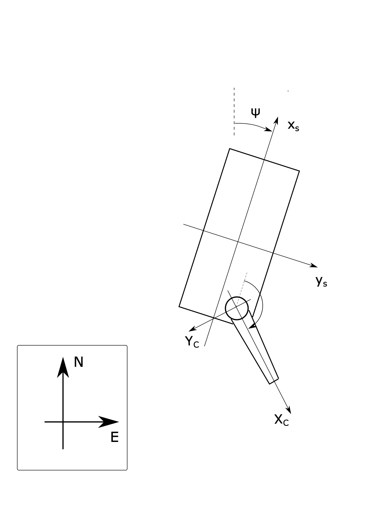
Fig. 12 A barge with a crane.

We also attach a reference system \(x_s, y_s, z_s\) (i.e., the \(s\)-frame) to the barge, as shown in the figure. The z-axis is pointing downwards in accordance with the right-hand rule. The location of the origin of the \(s\)-frame relative to the origin of the NED-frame is given as:

(125)\[\mathbf{r}_{s/n} = n \mathbf{i}_{n} + e \mathbf{j}_{n} + d \mathbf{k}_{n}\]

The position of the crane on the barge is given as:

(126)\[\mathbf{r}_{c/s} = a \mathbf{i}_{s} + b \mathbf{j}_{s} + c \mathbf{k}_{s}\]

The angle between the \(x_s\)-axis and the \(x_c\)-axis is \(\alpha\).

Finally, the distance from the origin of the crane-fixed reference frame to the tip of the crane is \(l\).

Note

When we ask for a vector in this problem, your answer should be in the form:

(127)\[\mathbf{r} = g \mathbf{i}_{k} + h \mathbf{j}_{k}\]

or:

(128)\[\begin{split}\mathbf{r}^k = \begin{bmatrix} g \\ h \end{bmatrix}\end{split}\]

where we need expressions for \(g\) and \(h\).

The expressions should be formulated in terms of the parameters \((a, b, c, l)\) , the variables \((\psi, \alpha, n, e, d)\) and their time derivatives \((\dot{\psi}, \dot{\alpha}, \dot{n}, \dot{e}, \dot{d})\).

Tasks

1. Find an expression for the position of the origin of the barge-fixed reference frame relative to the origin of the NED-frame expressed in terms of the barge-fixed reference frame.

2. Find an expression for the position of the tip of the crane relative to the origin of the \(s\)-frame as a function of \(\alpha\). Express the vector in terms of the \(s\)-frame.

3. Find an expression for the position of the tip of the crane relative to the origin of the NED-frame. Express the vector in terms of the NED-frame.

4. What is the angular velocity of the crane when the barge has a turn rate of \(\dot{\psi}\) and the crane base is rotating at the rate \(\dot{\alpha}\)?

5. The vessel has a forward velocity \(u\) and a sideways velocity of \(v\) relative to the inertial reference frame (the NED-frame). Find expressions for \(\dot{n}\) and \(\dot{e}\) (i.e., the time derivatives of the components in the equation above).

6. What is the linear velocity of the crane tip? The vessel still moves with a forward velocity component \(u\) and a sideways velocity component \(v\), and in addition, it has an angular speed of magnitude \(\dot{\psi}\). The crane has an angular speed with magnitude \(\dot{\alpha}\). You can express the answer in terms of the NED-frame.

Problem 3 - Parameterizations of Rotations

Fig. 13 ZYX Euler Angles as three successive rotations around the intermediate \(z\), \(y\) and \(x\) axes.

The ZYX Euler Angles is a parameterization of a rotation using three successive transformations around the intermediate \(z\), \(y\) and \(x\) axes (see Fig. 13). That is, the rotation matrix is given by

(129)\[\mathbf{R}_{\mathcal{B}}^{\mathcal{A}}(\theta,\phi,\psi) = \mathbf{R}_z(\psi) \mathbf{R}_y(\phi) \mathbf{R}_x(\theta)\]

where \(\mathbf{R}_x\), \(\mathbf{R}_y\), and \(\mathbf{R}_z\) represent the rotation matrix of the principal rotations around the \(z\), \(y\) and \(x\) axes, respectively.

(130)\[\begin{split}\boldsymbol{\chi} = \begin{bmatrix} \theta \\ \phi \\ \psi \end{bmatrix}\end{split}\]

are called the Euler Angles.

Tasks

1. Find the intermediate rotation matrices \(\mathbf{R}_{1}^{\mathcal{A}}\), \(\mathbf{R}_{2}^{1}\), and \(\mathbf{R}_{\mathcal{B}}^{2}\) along with the relative angular velocities expressed in the local frame \(\boldsymbol{\omega}_{1/\mathcal{A}}^{\mathcal{A}}\), \(\boldsymbol{\omega}_{2/1}^{1}\), and \(\boldsymbol{\omega}_{\mathcal{B}/2}^{2}\).

2. Show that the angular velocity of frame \(\mathcal{B}\) with respect to \(\mathcal{A}\) expressed in frame \(\mathcal{A}\) is given by

(131)\[\boldsymbol{\omega}_{\mathcal{B}/\mathcal{A}}^{\mathcal{A}} = \mathbf{E} \dot{\boldsymbol{\chi}}\]

where

(132)\[\begin{split}\mathbf{E} = \left[\begin{array}{ccc} \cos (\phi) \cos (\psi) & -\sin (\psi) & 0 \\ \cos (\phi) \sin (\psi) &\cos (\psi) & 0\\ -\sin (\phi) & 0 & 1 \end{array}\right]\end{split}\]

3. Show that the transformation \(\mathbf{E}\) is singular at \(\phi = \frac{\pi}{2} + k\pi\), \(\forall k \in \mathbb{Z}\). Why does this make Euler Angles a bad choice when modelling rotating systems that can reach any orientation? What parameterization, which tackles this issue, is usually preferred?

Problem 4 - Linked Mechanism

Fig. 14 Linked mechanism

The linked mechanism in Fig. 14 consists of the two rigid bodies AB and BC. Body AB rotates about the \(z_0\)-axis at a rate \(\dot{q}_1\), and body BC rotates about the \(y_2\)-axis at the rate \(\dot{q}_2\). The \(z_0\)-axis is parallel to the \(z_1\)-axis. The \(y_2\)-axis is parallel to the \(y_1\)-axis.

Hint

Use SymPy reference frames to solve the following problems.

Tasks

1. Find the position of the points B and C relative to point A, expressed in terms of the reference frame \(x_0y_0z_0\). The positions should be expressed as functions of \(\boldsymbol{q} = [q_1,\, q_2]^T\).

2. Find the angular velocity of the bodies AB and BC, expressed in terms of the reference frame \(x_0y_0z_0\).

3. Find the linear velocity of the points B and C, expressed in terms of the reference frame \(x_0y_0z_0\).

4. Express the linear velocity of point C in the form \(\boldsymbol{v}_C = \boldsymbol{J}(\boldsymbol{q})\dot{\boldsymbol{q}}\).

Problem 5 (optional) - Pendulum on rotating disk

Fig. 15 Pendulum on a rotating disk

The pendulum system shown in Fig. 15 consists of a flat surface, a disk that can roll on the surface, and a pendulum attached to the rim of the disk.

We have attached an inertial reference frame \(\theta\) such that the \(x_0\)-axis is aligned with the surface. We also have a moving reference frame at the center of the wheel. This reference frame will rotate with the wheel. Finally, we have attached a third reference frame to the hinge point of the pendulum such that the \(y_2\)-axis always remains aligned with the pendulum rod. Note that the angle \(\theta\) of the pendulum rod is given in terms of an axis that remains horizontal. You can assume no slip between the rim and the surface.

Hint

Equations 6.409 and 6.410 at page 261 in Egeland [Ege02], or Equations 60 and 77 in Rokseth and Gros [RG25], might be useful.

Tasks

1. Find the linear (translational) velocity of point A. Your answer should be expressed in terms of the parameters of the system, and the variables \(\phi\) and \(\theta\) and their time derivatives.

2. Find the linear acceleration of the point A of the parameters of the system, and the variables \(\phi\) and \(\theta\) and their first and second order time derivatives.