Pendulum Simulation

In this session, we will simulate the motion of a simple pendulum using the Forward Euler method. We will define system parameters, simulate its motion, and visualize the results.

1. Define the System Parameters

The system parameters include the mass of the pendulum, the length of the rod, gravitational acceleration, and optional damping.

import numpy as np

g = 9.8
r = 1

2. Define the Simulation Parameters

Simulation parameters define how the simulation is executed, such as the time step for the numerical method and the total simulation time.

time = 0
sim_time = 20
dt = 0.01

3. Prepare Data Storage

To analyze and visualize the simulation, we will store the system’s state (e.g., angular displacement and velocity) at each time step.

theta_data = []
omega_data = []
time_data = []

4. Define Initial Conditions

The initial conditions determine the starting state of the pendulum, such as its initial angle and angular velocity.

theta = 0
omega = 10

# Store data for initial time step
theta_data.append(theta)
omega_data.append(omega)
time_data.append(time)

5. Write the Forward Euler Solver

The Forward Euler method is a simple numerical technique to approximate solutions to differential equations. We will use it to update the system’s state step by step.

i = 0
while time <= sim_time:
    theta = theta_data[i] + omega_data[i] * dt
    omega = omega_data[i] + (-g/r * np.cos(theta_data[i]) - 0.1*omega_data[i])*dt


    # Progress time
    time = time + dt
    i = i+1

    # Store data for initial time step
    theta_data.append(theta)
    omega_data.append(omega)
    time_data.append(time)

Note

During the lecture, I did not implement the forward Euler equation correctly.I used the newly updated \(\theta\) to update the \(\omega\)-equation, rather than the previous value.

I have updated this by pulling the previous value $ \theta`(t_i) $ instead of $ :nbsphinx-math:theta`(t_{i+1}) $ from the stored data.

6. Visualize the Results

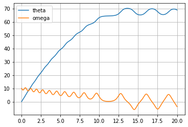
Visualization helps us understand the dynamics of the system. We will plot the angular displacement over time and the phase space trajectory.

import matplotlib.pyplot as plt

plt.plot(time_data, theta_data, label="theta")
plt.plot(time_data, omega_data, label="omega")
plt.legend()
plt.grid(True)
plt.show()

7. Conclusion and Discussion

Summarize the key points of the session and explore further ideas such as adding damping or changing the time step.